"""
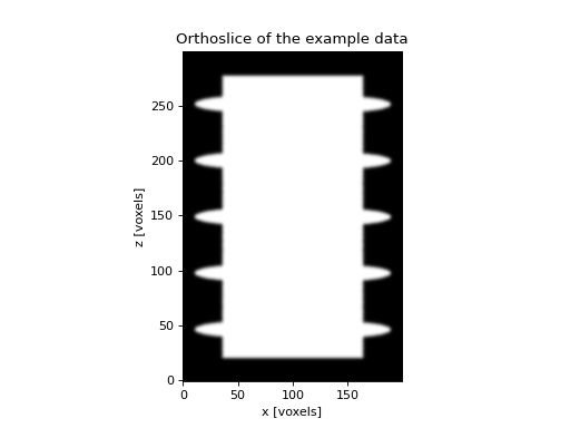
In this example I will show what a standard analysis workflow looks like. For
the example I will use a right-handed helical shape that consists of an achiral
core surrounded by two helices from the file ``helix.npy``. This shape is
already pre-aligned, so the alignment steps are not necessary, but for the
purpose of this example I will nevertheless show how to use them.
"""
import numpy as np
import matplotlib.pyplot as plt
import heliq
# First we need to load the data, it is up to you to load your data from any
# file type you want to use. For this example I stored the data with numpy. It
# is important to know that the data should be a 3D numpy array of which the
# first axis corresponds to the real-world y-axis, the second axis to the real
# x-axis, and the third axis to the z-axis. This is the commonly used
# rows-columns-channels convention. You also need to know the width of the
# voxels to be able to compare the helicity of different samples recorded with
# different settings. For the purpose of this example, I'll use a voxel size of
# one.
data = np.load("helix.npy")
voxel_size = 1.0
_, ax = plt.subplots(1, 1)
ax.imshow(data[:, data.shape[1]//2, :].T, cmap='gray', origin='lower')
ax.set_title("Orthoslice of the example data")
ax.set_xlabel("x [voxels]")
ax.set_ylabel("z [voxels]")
# The data needs to be aligned such that the helical axis is in the center and
# parallel to the z-axis. For typical elongated shapes, this can be done by
# aligning the longest axis with the z-axis and moving the center of mass to
# the center of the data. For atypical shapes you might have to do this
# manually.
center = heliq.center_of_mass(data)
orientation = heliq.helical_axis_pca(data, 0)
data = heliq.align_helical_axis(data, orientation, center)
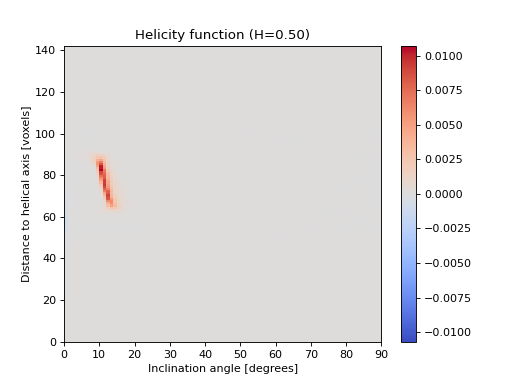
# Next you can calculate the helicity. The helicity function gives a 2D
# histogram that shows the distribution of helical features in the data as
# function of their inclination angle (alpha) and distance to the helical axis
# (rho). Note that the voxel size is important to be able to compare the
# results of different shapes. Negative values represent left-handed helicity
# and positive values indicate right-handed helicity. The total helicity is a
# value between -1 and 1 that gives an idea of the helicity of the entire
# shape.
hfunc = heliq.helicity_function(data, voxel_size)
htot = heliq.total_helicity(hfunc)
# To plot the helicity function, you can use the following function, which will
# apply a diverging colormap and set the intensity limits appropriatly. You do
# have to call ``plt.show()`` at the end of your script though!
fig, ax = plt.subplots(1, 1)
im = heliq.plot_helicity_function(hfunc, axis=ax)
fig.colorbar(im)
ax.set_title(f"Helicity function (H={htot:0.2f})")
ax.set_xlabel("Inclination angle [degrees]")
ax.set_ylabel("Distance to helical axis [voxels]")
# You can also create a helicity map, which is a 3D numpy array that indicates
# the location of right- and left-handed helical features. The argument
# ``sigma`` needs to be chosen manually according to the expected size of the
# helical features.
hmap = heliq.helicity_map(data, sigma=5)
fig, ax = plt.subplots(1, 1)
im = ax.imshow(hmap[:, hmap.shape[1]//2, :].T, cmap='coolwarm', origin='lower')
ax.set_title("Orthoslice of the helicity map")
ax.set_xlabel("x [voxels]")
ax.set_ylabel("z [voxels]")
vmax = np.max(np.abs(hmap))
im.set_clim(-vmax, vmax)
fig.colorbar(im)
plt.show()
